Constraining VNS tomographic inversions using an SWI model
This walkthrough assumes the following:
- A Merge has been created
- First break picks are available
- An SWI model has already been generated
Create a new VNS tomography model
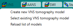
Open the Merge window and select “VNS” followed by “Create new VNS tomography model”:
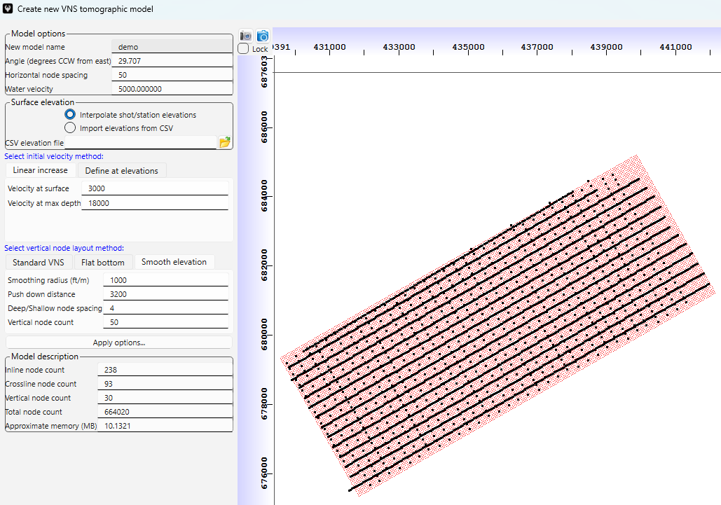
The initial velocity field is unimportant since it will be overridden in the next steps. The default vertical node count has been increased to 50 from 30, and the deep/shallow node spacing has been increased to 4. These changes will help incorporate the SWI model.
Initialize the velocity field using the moveout trend curves (optional)
Initializing the VNS velocity field with a field generated from the trend curves can significantly speed up the tomographic inversion. The shallowest layers will be overridden in the next step.
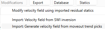
Click “Modifications” followed by “Import: Generate velocity field from moveout trend picks”:
Aside – the velocity field is generated using a 1-D Eikonal solver to fit the trend picks ay each picked location.
Import the SWI model into the VNS model
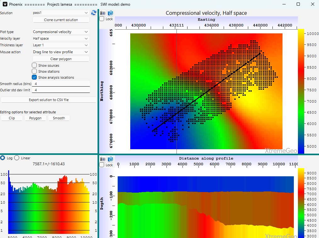
Here is a profile of the SWI model we’re going to use (bottom plot), along with the half-space velocity (top plot). Note that the half-space boundary is at about 300 feet of depth.
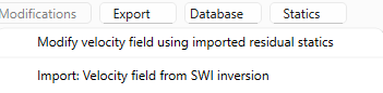
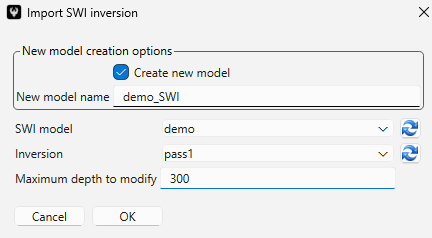
Navigate back to the VNS model window and select “Modifications:” followed by “Import: Velocity field from SWI inversion”
Select the correct SWI model and inversion. In this case we’re going to use the SWI model to modify the upper 300 feet of the VNS model:
Define the constraint (AKA the “blend”) function
The spatially varying constraint field is a 3D volume of floating point numbers that range between 0 and 1.
- X is a 3D vector
- Let VC(X) be the user-defined constraining velocity function. This is what we created by importing the SWI velocity field.
- Let B(X) be the user-defined blending function (between 0 and 1)
- Set VI(X) = VC(X)
- Inversion loop step 1: V_OUT(X) = Single-loop tomographic inversion of VI(X)
- Inversion loop step 2: OUTPUT(X) = VC(X) * B(X) + (1 – B(X)) * V_OUT(X)
- Inversion loop step 3: Set VI(X) = OUTPUT(X)
- Inversion loop step 4: Go back to step 1 until all loops (usually 15 or 20) done
- Inversion loop step 5: Final result = OUTPUT(X)
- Select “Constraint” followed by “Blending function: set to constant”. Enter the value “0.0” and click “ok”.
- Select “Constraint” then “Blending function: Layer method”
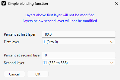
The above options put a very strong constraint on the top layer tapering down to zero at depth around 330 feet. At this point you should view the blending function on a profile to make sure it’s okay.
Run the tomographic update
Start the inversion as usual – select “Analysis” then “Model update – standard approach”.
Be sure to allow velocity inversions – uncheck “Force velocity to increase with depth”.
Enter your desired values in the wizard until you reach this page:
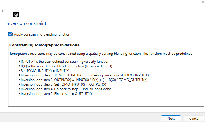
Be sure to check “Apply constraining blending function”! And that’s it. Finish the wizard and start the job.